If you're reading this article, it looks like you're wondering how you can better optimize your Redshift queries - and you're probably wondering how you can do that in conjunction with dbt.

In order to properly optimize, we need to understand why we might be seeing issues with our performance and how we can fix these with dbt sort and dist configurations.

In this article, we’ll cover:

• A simplified explanation of how Redshift clusters work
• What distribution styles are and what they mean
• Where to use distribution styles and the tradeoffs
• What sort keys are and how to use them
• How to use all these concepts to optimize your dbt models.

Let’s fix this once and for all!

The Redshift cluster

In order to understand how we should model in dbt for optimal performance on Redshift, I’m first going to step through a simplified explanation of the underlying architecture so that we can set up our examples for distributing and sorting.

First, let’s visualize an example cluster:

This cluster has two nodes, which serve the purpose of storing data and computing some parts of your queries. You could have more than this, but for simplicity we’ll keep it at two.

These two nodes are like the office spaces of two different people who have been assigned a portion of work for the same assignment based on the information they have in their respective offices. Upon completion of their work, they give their results back to their boss who then assembles the deliverable items and reports the combined information back to the stakeholder.

Let's look at the data waiting to be loaded into Redshift:

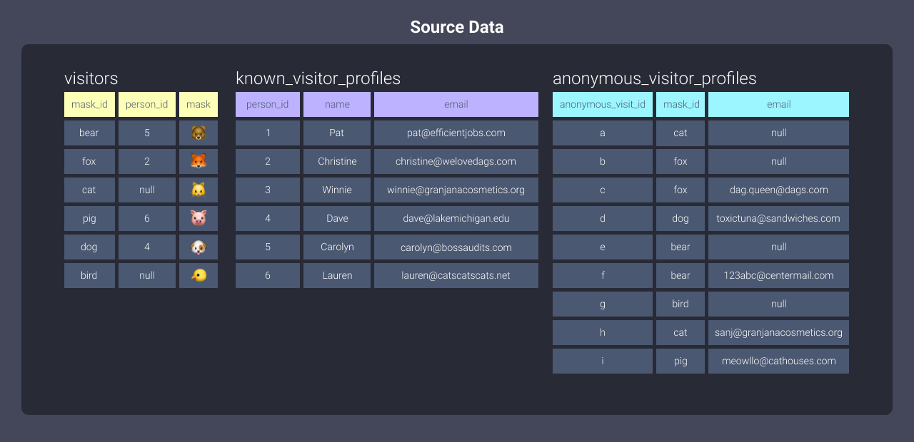
You can see there are three tables of data here. When you load data into Redshift, the data gets distributed between the offices. In order to understand how that happens, let’s take a look at distribution styles.

What are distribution styles?

Distribution styles determine how data will be stored between offices (our nodes). Redshift has three distribution styles:

• all
• even
• key-based

Let’s dive into what these mean and how they work.

The all distribution style

An all distribution means that both workers get the same copies of data. To implement this distribution on our tables in dbt, we would apply this configuration to each of our models:

{{ config(materialized='table', dist='all') }}

Here's a visualization of the data stored on our nodes:

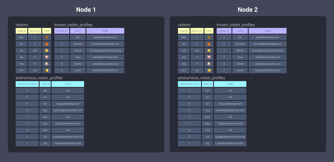
When to use the all distribution:

This type of distribution is great for smaller data which doesn’t update frequently. Because all puts copies of our tables on all of our nodes, we’ll want to be sure we’re not giving our cluster extra work by needing to do this frequently.

The even distribution style

An even distribution means that both workers get close to equal amounts of data distributed to them. Redshift does this in a round-robin playing card style.

To implement this distribution on our tables in dbt, we would apply this configuration to each of our models:

{{ config(materialized='table', dist='even') }}

Here's a visualization of the data stored on our nodes:

Notice how our first worker received the first rows of our data, the second worker received the second rows, the first worker received the third rows, etc.

When to use the even distribution

This distribution type is great for a well-rounded workload by ensuring that each node has equal amounts of data. We’re not picky about which data each node handles, so the data can be evenly split between the nodes. That also means an equal amount of assignments are passed out resulting in no capacity wasted.

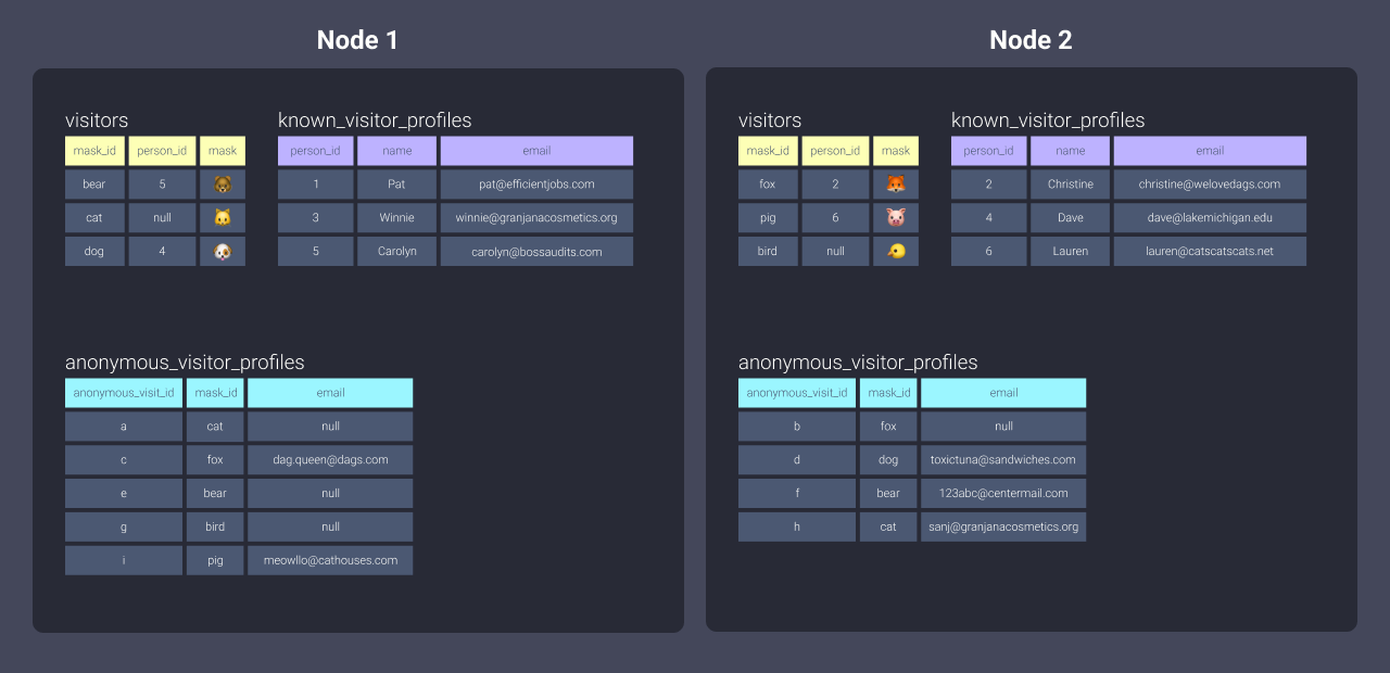
The key-based distribution style

A key-based distribution means that each worker is assigned data based on a specific identifying value.

Let's distribute our known_visitor_profiles table by person_id by applying this configuration to the top of the model in dbt:

{{ config(materialized='table', dist='person_id') }}

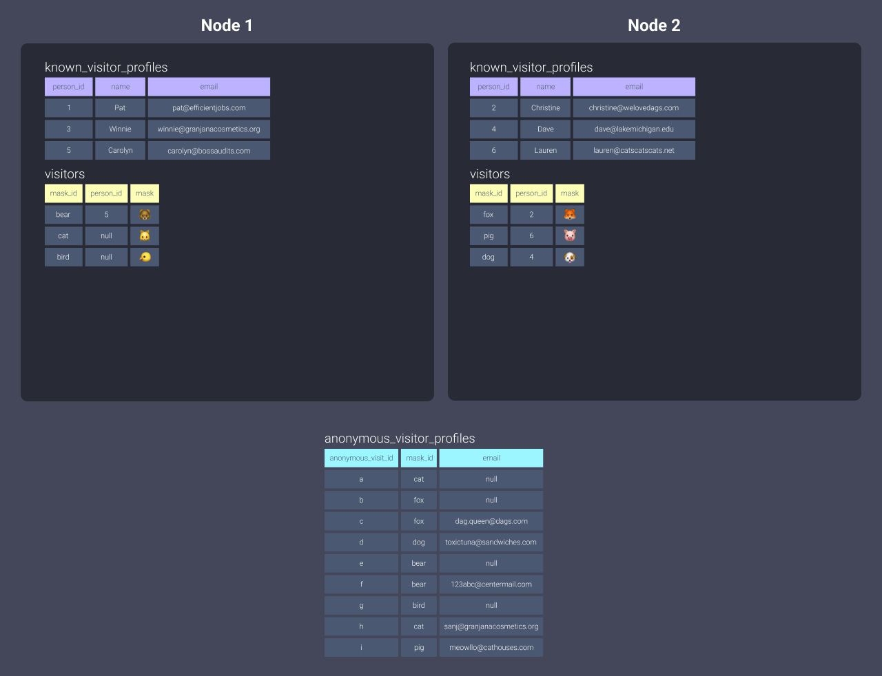
Here's a visualization of the data stored on our nodes:

It doesn’t look that different from even, right? The difference here is that because we’re using person_id as our distribution key, we ensure:

• Node 1 will always get data associated with values 1, 3, 5
• Node 2 will always get data associated with values 2, 4, 6

Let’s do this with another table to really see the effects. We'll apply the following configuration to our visitors.sql file:

{{ config(materialized='table', dist='person_id') }}

Here's a visualization of the data stored on our nodes:

You can see above that because we distributed visitors on person_id as well, the nodes received the associated data we outlined above. We did have some null person_ids - those will be treated as a key value and distributed to one node.

When to use key-based distribution

Key-based distribution is great for when you’re really stepping it up. If we can dial in to our commonly joined data, then we can leverage the benefits of co-locating the data on the same node. This means our worker can have the data they need to complete the tasks they have without duplicating the amount of storage we need.

Things to keep in mind when working with these configurations

Redshift has defaults.
Redshift initially assigns an all distribution to your data, but switches seamlessly to an even distribution based on the growth of your data. This gives you time to model out your data without worrying too much about optimization. Reference what you learned above when you’re ready to start tweaking your modeling flows!

Distribution only works on stored data.
These configurations don’t work on views or ephemeral models. This is because the data needs to be stored in order to be distributed. That means that the benefits only happen using table or incremental materializations.

Applying sort and distribution configurations from dbt doesn’t affect how your raw data is sorted and distributed.
Since dbt operates on top of raw data that’s already loaded into your warehouse, the following examples are geared towards optimizing your models created with dbt.

You can still use what you learn from this guide to choose how to optimize from ingestion, however this would need to be implemented via your loading mechanism. For example if you’re using a tool like Fivetran or Stitch, you’ll want to consult their docs to find out whether you can set the sort and distribution on load through their interfaces.

Redshift is a columnar-store database.
It doesn’t actually orient data values per row that it belongs to, but by column they belong to. This isn’t a necessary concept to understand for this guide, but in general columnar stores can be faster at retrieving data the more specific the selection you make. While being selective of columns can optimize your model, I’ve found that it doesn’t have as tremendous an impact most of the time as setting sort and distribution configs. As such, I won’t be covering this.

Handling joins: Where distribution styles shine

Distribution styles really come in handy when we’re handling joins. Let’s work with an example. Say we have this query:

select <your_list_of_columns>
from visitors
left join known_visitor_profiles
on visitors.person_id = known_visitor_profiles.person_id

Now let’s look at what Redshift does per distribution style if we distribute both tables the same way.

All

Using all copies our data sets and stores the entirety of each within each node.

In our offices example, that means our workers can do their load of the work in peace without being interrupted or needing to leave their office, since they each have all the information they need.

The con here is that every time data needs to be distributed, it takes extra time and effort - we need to run to the copy machine, print copies for everyone, and pass them out to each office. It also means we have 2x the paper!

This is fine if we have data that doesn’t update too frequently.

Even

Using even distributes our data sets as described in the What are Distribution Styles? section (round-robin) to each node. The even distribution results in each node having data that they may or may not need for their assigned tasks.

In our scenario of office workers, that means that if our workers can’t find the data they need to complete their assignment in their own office they need to send a request for information to the other office to try to locate the data. This communication takes time!

You can imagine how this would impact how long our query takes to complete. However, this distribution is usually a good starting point even with this impact because the workload to assemble data is shared in equal amounts and probably not too skewed - in other words, one worker isn’t sitting around with nothing to do while the other worker feverishly tries to work through stacks of information.

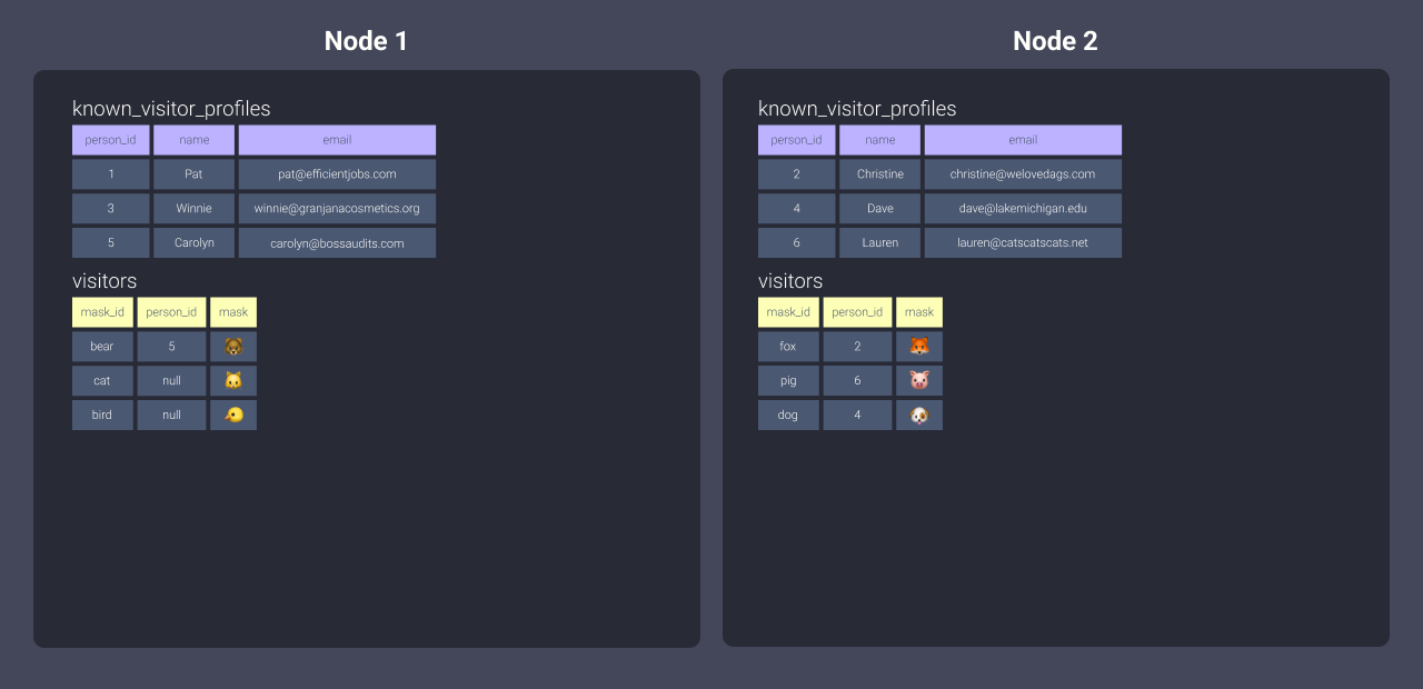
Key-based

Our key-based distribution of person_id gave our nodes assigned data to work with. Here’s a refresher from the What are Distribution Styles? section:

• Node 1 was distributed data associated with key values null, 1, 3, and 5.
• Node 2 was distributed data associated with key values 2, 4, and 6

This means that when we join the two tables we distributed, the data is co-located on the same node and therefore our workers don’t need leave their offices to collect the data they need to complete their work. Cool, huh?

Where it breaks down 🚒 🔥 👩🏻‍🚒

You would think the most ideal distribution would be key-based. However, you can only assign one key to distribute by and that means if we have a query like this, we run into issues again:

select <your_list_of_columns>
from visitors
left join known_visitor_profiles
    on visitors.person_id = known_visitor_profiles.person_id
left join unknown_visitor_profiles
    on visitors.mask_id = anonymous_visitor_profiles.mask_id

How would you decide to distribute the anonymous_visitor_profiles data?

We have a few options:

• Distribute by all
  But if it’s a table that updates frequently, this may not be the best route.

• Distribute by even
  But then our nodes need to communicate when visitors is joined to anonymous_visitor_profiles.

  If you decide to do something like this, you should consider what your largest datasets are first and distribute using appropriate keys to co-locate that data. Then, benchmark the run times with your additional tables distributed with all or even - the additional time may be something you can live with!

• Distribute by key
  Distributing the anonymous_visitor_profiles with a key in this situation won’t really do anything, since you’re not co-locating any data! For example, we could change to distribute by mask_id, but then we’d have to distribute the visitors table by mask_id and then you’d end up in the same boat again with the known_visitor_profiles model!

Thankfully with dbt, distributing isn’t our only option.

How to have your cake and eat it, too 🎂

Okay, so what if you want to have a key-based distribution, but you want to make those joins happen as well?

This is where the power of dbt modeling really comes in! dbt allows you to break apart your queries into things that make sense. With each query, you can assign your distribution keys to each model, meaning you can have much more control.

The following are some methods I’ve used in order to properly optimize run times, leveraging dbt’s ability to modularize models.

Note

I won’t get into our modeling methodology at dbt Labs in this article, but there are plenty of resources to understand what might be happening in the following DAGs!

Staggered joins

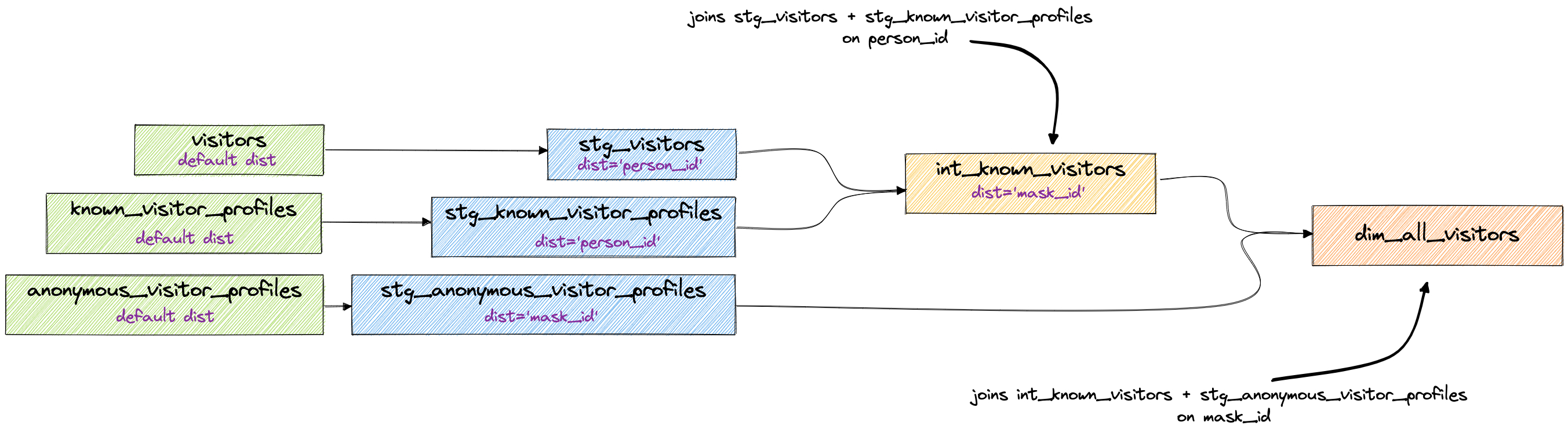
In this method, you piece out your joins based on the main table they’re joining to. For example, if you had five tables that were all joined using person_id, then you would stage your data (doing your clean up too, of course), distribute those by using dist='person_id', and then marry them up in some table downstream. Now with that new table, you can choose the next distribution key you’ll need for the next process that will happen. In our example above, the next step is joining to the anonymous_visitor_profiles table which is distributed by mask_id, so the results of our join should also distribute by mask_id.

Resolve to a single key

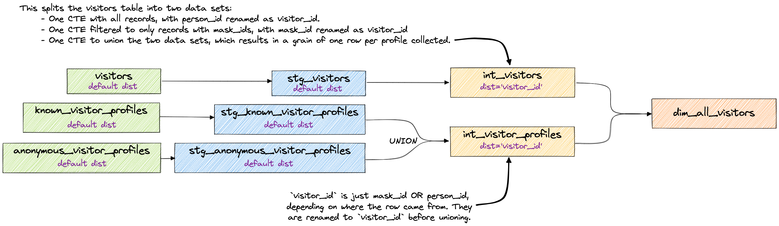
This method takes some time to think about, and it may not make sense to do it depending on what you need. This is definitely balance between coherence, usability, and performance.

The main point here is that you’re resolving the various keys and grains before the details are joined in. Because we’re not joining until the end, this means that only our intermediate tables get distributed based on the resolved keys and finally joined up in dim_all_visitors.

Sometimes the work you’re doing downstream is much easier to do when you do some complex modeling up front! When you want or need it, you’ll know.

Sort keys

Lastly, let’s talk about sort keys. No matter how we’ve distributed our data, we can define how data is sorted within our nodes. By setting a sort key, we’re telling Redshift to chunk our rows into blocks, which are then assigned a min and max value. Redshift can now use those min and max values to make an informed decision about which data it can skip scanning.

Imagine that our office workers have no organization taking place with their documents - the papers are just added in the order they’re given. Now imagine that each worker needs to retrieve all paperwork associated to the person who wore a dog mask to the party. They would need to thumb through every drawer and every paper in their filing cabinets in order to pull out and assemble the information related to the dog-masked person.

Let’s take a look at the information in our filing cabinet in both sorted and unsorted formats. Below is our anonymous_visitor_profiles table sorted by mask_id:

Once sorted, Redshift can keep track of what exists in blocks of information. This is equivalent to the information in our filing cabinet being organized into folders where items with mask ids starting with letters b through c are in located in one folder, mask ids starting with letters d through f are in another folder, and so on. Now our office worker can skip looking through the folder b-c and skip straight to d-f:

Even without setting an explicit distribution, this can help immensely with optimization. Here are some good places to apply it:

• On any model you expect to be frequently filtered by range.
• Your ending models (often referred to as marts). Your stakeholders will be using these to slice and dice data. It’s best to sort based on how the data is most often filtered (This is most likely dates or datetimes!)
• On frequently joined keys. Redshift suggests you distribute and sort by these, as it allows Redshift to execute a sort merge join in which the sorting phase gets bypassed.

Parting thoughts

Now that you know all about distribution, sorting, and how you can piece out your dbt models for better optimization, it should be much easier to make the decision on how to plan your optimization tactfully!

I have some ending thoughts before you get into tweaking these configurations:

Let Redshift do its thing

It’s nice to be able to sit back and watch how it performs without intervention! By allowing yourself the time to watch your models, you can be much more targeted with your optimization plans.

Document before tweaking

If you’re about to tweak these configurations, make sure you document how long the model takes before the changes! If you have dev limits in place, you can still run a benchmark against the limit before and after the tweaks, although it is more ideal to work with larger amounts of data to really understand how it would affect processing once in production. I’ve been able to successfully test tweaks on limited data sets and it’s translated beautifully within production environments, but your milage may vary.

Test removing legacy dist styles and sort keys first

If there are any sort keys or distribution styles already defined, remove those to see how your models do with the default. Having a bad sort key or distribution style can negatively impact your performance, which is why I suggest not configuring these on any net new modeling unless you’re sure about the impact.

Decide whether you you need to optimize at all!

Identifying whether you need to change these configurations sometimes isn’t straightforward, especially when you have a lot going on in your model! Here’s some tips to help you out:

• Use the query optimizer
  If you have access to look at Redshift’s query optimizer in the Redshift console or have permissions to run an explain/explain analyze yourself, it can be helpful in drilling down to problematic areas.

• Organize with CTEs
  You know we love CTEs - and in this instance they really help! I usually start troubleshooting a complex query by stepping through the CTEs of the problematic model. If the CTEs are executing logic in nicely rounded ways, it’s easy to find out which joins or statements are causing the issues.

• Look for ways to clean up logic
  This can be things like too much logic used on a join key, a model handling too many transformations, or bad materialization assignments. Sometimes all you need is a little code cleanup!

• Step through joins one at a time
  If it's one join, it’s easy to understand which keys to optimize by. If there’s multiple joins, you might need to comment out joins in order to understand which present the most problems. It’s a good idea to benchmark each approach you take.

  Here’s an example workflow:

  1. Run the problematic model (I do this a couple of times to get a baseline average on runtime). Notate the build time.
  2. Comment out joins and one by one, run the model. Keep doing this until you find which join is causing unideal run times.
  3. Decide on how best to optimize the join:
     • Optimize the logic or flow, such as moving the calculation on a key to a prior CTE or upstream model before the join.
     • Optimizing the distribution, such as doing the join in an upstream model so you can facilitate co-location of the data.
     • Optimizing the sort, such as identifying and assigning a frequently filtered column so that finding data is faster in downstream processing.

Now you have a better understanding of how to leverage Redshift sort and distribution configurations in conjunction with dbt modeling to alleviate your modeling woes.

If you have any more questions about Redshift and dbt, the #db-redshift channel in dbt’s community Slack is a great resource.

Now get out there and optimize! 😊