

When running a job that has over 1,700 models, how do you know what a “good” runtime is? If the total process takes 3 hours, is that fantastic or terrible? While there are many possible answers depending on dataset size, complexity of modeling, and historical run times, the crux of the matter is normally “did you hit your SLAs”? However, in the cloud computing world where bills are based on usage, the question is really “did you hit your SLAs and stay within budget”?
Here at dbt Labs, we used the Model Timing tab in our internal analytics dbt project to help us identify inefficiencies in our incremental dbt Cloud job that eventually led to major financial savings, and a path forward for periodic improvement checks.
Your new best friend: The Model Timing tab
The dbt Labs internal project is a beast! Our daily incremental dbt Cloud job runs 4x/day and invokes over 1,700 models. We like to sift through our dbt Cloud job using the Model Timing tab in dbt Cloud. The Model Timing dashboard displays the model composition, order, and run time for every job run in dbt Cloud (for team and enterprise plans). The top 1% of model durations are automatically highlighted, which makes it easy to find bottlenecks in our runs. You can see that our longest running model stuck out like a sore thumb -- here's an example of our incremental job before a fix was applied:
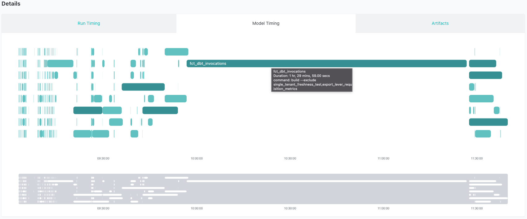
As you can see, it's straightforward to identify the model that's causing the long run times and holding up other models. The model fct_dbt_invocations takes, on average, 1.5 hours to run. This isn't surprising, given that it's a relatively large dataset (~5B records) and that we're performing several intense SQL calculations. Additionally, this model calls an ephemeral model named dbt_model_summary that also does some heavy lifting. Still, we decided to explore if we could refactor this model and make it faster.
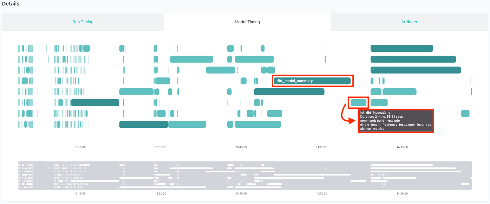
After refactoring this code, we ended up swapping the ephemeral model dbt_model_summary to an incremental model that took the bulk of the processing out of the main fct_dbt_invocations model. Instead of recalculating this complex logic every run, we pull only new data and run that logic on the smaller subset of those records. The combined run time of the new dbt_model_summary and fct_dbt_invocations is now ~15-20 minutes, a savings of over an hour per run!
Identifying the problem
This project runs on Snowflake, so all the examples below show the Snowflake UI. However, it is possible to do a similar style of analysis in any data warehouse.
Also, this blog post represents a pretty technical deep dive. If everything you read here doesn't line up immediately, that's ok! We recommend reading through this article, then brushing up on cloud data warehouses and query optimization to help supplement the learnings here.
Unpacking the query plan
Finding this long running query was step one. Since it was so dominant in the Model Timing tab, it was easy to go straight to the problematic model and start looking for ways to improve it. The next step was to check out what the Snowflake query plan looked like.
There are a few ways you can do this: either find the executed query in the History tab of the Snowflake UI, or grab the compiled code from dbt and run it in a worksheet. As it’s running, you can click on the Query ID link to see the plan. More details on this process are available in your provider’s documentation (Snowflake, BigQuery, Redshift, Databricks).
Below you can see the query plan for fct_dbt_invocations, which includes the logic from dbt_model_summary:
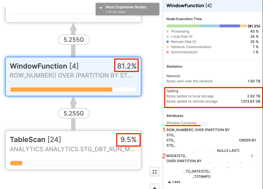
From the query profile, it was easy to find the issue. There are two window functions that account for over 90% of the run time when we factor in the table scan needed to retrieve the data. Additionally, there is nearly 1TB worth of data that is spilled to remote storage as part of this query. Within Snowflake, remote storage is considerably slower to both write and read from, so any data that’s on the remote drive will really slow down a query. We’ve found the problem!
Understanding the data
Once we identified the issue, we had to find a way to fix it.
First, it’s good to have a high level understanding of the underlying data for fct_dbt_invocations. Any time you issue a command to dbt (run, test, build, snapshot, etc.), we track certain pieces of metadata about that run. We call these “invocations,” and as you can imagine, dbt is invoked a lot. The table this query is running against is filtered, but still has somewhere in the neighborhood of 5 billion rows. The relevant pieces of data that we are using in this query include project IDs, model IDs, and an anonymized hash key representing the raw model contents to know if a model changed.
If you’re curious, here’s a look at the query for dbt_model_summary before any changes were made:
{{config(materialized = 'ephemeral')}}

with model_execution as (

    select * from {{ ref('stg_dbt_run_model_events') }}

),

diffed as (

    select *,

        row_number() over (
            partition by project_id, model_id
            order by dvce_created_tstamp
        ) = 1 as is_new,

        /*
            The `mode` window function returns the most common content hash for a
            given model on a given day. We use this a proxy for the 'production'
            version of the model, running in deployment. When a different hash
            is run, it likely reflects that the model is undergoing development.
        */

        contents != mode(contents) over (
            partition by project_id, model_id, dvce_created_tstamp::date
        ) as is_changed

    from model_execution

),

final as (

    select
        invocation_id,
        max(model_complexity) as model_complexity,
        max(model_total) as count_models,
        sum(case when is_new or is_changed then 1 else 0 end) as count_changed,
        sum(case when skipped = true then 1 else 0 end) as count_skip,
        sum(case when error is null or error = 'false' then 0 else 1 end) as count_error,
        sum(case when (error is null or error = 'false') and skipped = false then 1 else 0 end) as count_succeed

    from diffed
    group by 1

)

select * from final
The window functions referenced above are answering the following questions:
row_number()- Is this the first time that this specific model has run in a project?
- Note: this grain is at the project level
mode()- Is this the most frequent version of the model that ran today (based on the hashed contents)?
- Note: this grain is at the model + run date level
Moving to solutions
Attempt #1: Optimizing our objects and materializations
Given the size and complexity of this query, the first few approaches we took didn’t focus on changing the query as much as optimizing our objects and materializations.
The two window functions (row_number() and mode() in the diffed CTE above) were in an ephemeral model which isn’t stored in the data warehouse, but is instead executed in-memory at run time. Since it was obvious our virtual warehouse was running out of memory (remote storage spillage), we tried swapping that to a view, then a table materialization. Neither of these improved the run time significantly, so we tried clustering the table. However, since our two window functions are at different grains there wasn’t a great clustering key we found for this.
Attempt #2: Moving to an incremental model
The final strategy we tried, which ended up being the solution we implemented, was to swap the ephemeral model (dbt_model_summary) to an incremental model. Since we’re calculating metrics based on historical events (first model run, most frequent model run today), an incremental model let us perform the calculation for all of history once in an initial build, then every subsequent build only needs to look at a much smaller subset of the data to run it’s calculations.
One of the biggest problems with the ephemeral model was remote spillage due to lack of memory, so having a smaller dataset to run the calculation against made a massive impact. Snowflake can easily calculate a daily mode or a first model run when we only had to look at a sliver of the data each time.
Swapping from ephemeral to incremental can be simple, but in this case we are calculating at two grains and need more than just the data loaded since the prior run.
row_number()- To get the first time a model was run, we need every invocation of that model to see if this is the first one. Still, we don’t need the full history, just the subset that changed today. This is handled in the
new_modelsCTE you can see below.
- To get the first time a model was run, we need every invocation of that model to see if this is the first one. Still, we don’t need the full history, just the subset that changed today. This is handled in the
mode()- Since we’re calculating a daily mode, we actually need the full day’s worth of data every time this incremental model runs. We do that by applying the
::dateoperator to our incremental logic to always pull a full days (or multiple days) worth of history each time.
- Since we’re calculating a daily mode, we actually need the full day’s worth of data every time this incremental model runs. We do that by applying the
This let to slightly more complex logic in the model, as you can see below:
{{config(materialized = 'incremental', unique_key = 'invocation_id')}}

with model_execution as (

    select *
    from {{ ref('stg_dbt_run_model_events') }}
    where
        1=1
    {% if target.name == 'dev' %}

        and collector_tstamp >= dateadd(d, -{{var('testing_days_of_data')}}, current_date)

    {% elif is_incremental() %}

        --incremental runs re-process a full day everytime to get an accurate mode below
        and collector_tstamp > (select max(max_collector_tstamp)::date from {{ this }})

    {% endif %}

),

{# When running rull refresh we have access to all records, so this logis isn't needed #}
{% if is_incremental() %}
new_models as (

    select
        project_id,
        model_id,
        invocation_id,
        dvce_created_tstamp,
        true as is_new
    from {{ ref('stg_dbt_run_model_events') }} as base_table
    where
        exists (
                select 1
                from model_execution
                where
                    base_table.project_id = model_execution.project_id
                    and base_table.model_id = model_execution.model_id
            )
    qualify
        row_number() over(partition by project_id, model_id order by dvce_created_tstamp) = 1


),
{% endif %}

diffed as (

    select model_execution.*,

        {% if is_incremental() %}

            new_models.is_new,

        {% else %}

            row_number() over (
                partition by project_id, model_id
                order by dvce_created_tstamp
            ) = 1 as is_new,

        {% endif %}

        /*
            The `mode` window function returns the most common content hash for a
            given model on a given day. We use this a proxy for the 'production'
            version of the model, running in deployment. When a different hash
            is run, it likely reflects that the model is undergoing development.
        */

        model_execution.contents != mode(model_execution.contents) over (
            partition by model_execution.project_id, model_execution.model_id, model_execution.dvce_created_tstamp::date
        ) as is_changed

    from model_execution
        {% if is_incremental() %}
            left join new_models on
                model_execution.project_id = new_models.project_id
                and model_execution.model_id = new_models.model_id
                and model_execution.invocation_id = new_models.invocation_id
                and model_execution.dvce_created_tstamp = new_models.dvce_created_tstamp
        {% endif %}

),

final as (

    select
        invocation_id,
        max(collector_tstamp) as max_collector_tstamp,
        max(model_complexity) as model_complexity,
        max(model_total) as count_models,
        sum(case when is_new or is_changed then 1 else 0 end) as count_changed,
        sum(case when skipped = true then 1 else 0 end) as count_skip,
        sum(case when error is null or error = 'false' then 0 else 1 end) as count_error,
        sum(case when (error is null or error = 'false') and skipped = false then 1 else 0 end) as count_succeed

    from diffed
    group by 1

)

select * from final
The astute reader will notice that the entire new_models CTE is wrapped in an {% if is_incremental() %} block. That’s because when the model is ran incrementally we need the full history of model runs for the given model. This means we have to join back to the main table to get that full history. However, when we’re running this as a full refresh (or on the initial load), we already have the full history of runs in the query, so we don’t need to join back to the table. This additional piece of {% if is_incremental() %} dropped the full refresh run time down from over 2 hours to just under 30 minutes. This is a one time savings (or however often we have to full refresh), but is well worth the slightly more complex logic.
Difficulty with testing
A major challenge in testing and implementing our changes was the volume of data needed for comparison testing. Again, the biggest problem we had was that our virtual warehouse was running out of memory, so trying to do performance testing on a subset of the data had misleading results (our testing was a subset of 10 million records). Since this query runs just fine on a small set of data (think the incremental runs), when we were initially trying to performance test the new vs old it looked like there was no real benefit to the incremental model. This led to many wasted hours of trying to figure out why we weren’t seeing an improvement.
Eventually, we figured out that we needed to test this on the full dataset to see the impact. In the cloud warehousing world where you pay-for-use this has very easy to track cost implications. However, you have to spend money to make money, so we decided the increased cost associated with testing this on the full dataset was worth the expense.
To start with, we cloned the entire prod schema to a testing schema, which is a free operation in Snowflake. Then, we did an initial build of the new dbt_model_summary model since it was switching from ephemeral to incremental. Once that was complete, we were able to delete out a few days worth of data from both dbt_model_summary and fct_dbt_invocations to see how long an incremental run would take. This represented the true day-to-day runs, and the results were fantastic! The combined run time of both models dropped from 1.5 hours to 15-20 minutes for incremental runs.
Benefits of the improvement
The end result of this improvement saves a nice chunk of change. Since this query was running 4 times per day and took 1.5 hours per run, this change is saving roughly 5 hours per day in run time. Given that this on Snowflake, we can calculate the savings based on their public pricing. Currently for the Enterprise edition of Snowflake it costs $3/credit, and a medium warehouse consumes 4 credits/hour. Putting this all together, that’s a savings of ~$1800/month.
The cost savings are great, but there are two other “time based” benefits that come from faster runs:
- Since this process runs 4 times daily, there is a limit to the length any given run can take, and in turn how many metrics we can calculate. By saving time on the longest running metrics it frees up runtime for us to add new logic to our runs. This generally leads to happier end consumers because they get more information to work with.
- If the need ever arises to refresh our data more frequently, we now have some runway to do that. While these particular models will never be near-real-time, we could realistically get more up-to-date information since we can now process the data faster.
Conclusion
Developing an analytic code base is an ever-evolving process. What worked well when the dataset was a few million records may not work as well on billions of records. As your code base and data evolve, be on the lookout for areas of improvement. This article showed a very specific example around two models, but the general principals can be applied to any code base:
Periodically review your run times
This is made easy with the Model Timing tab in dbt Cloud. You can quickly go to any run to see the model composition, order, and run time for every run in dbt Cloud. The longest running models stick out like a sore thumb!
Use the query analyzer from your data warehouse
Once you’ve found the problematic model (or models!), use the query analyzer to find which part of the model takes the longest to run. The graphical tree provided gives you a more fine grained view into what is going on. Some tips to look out for:
- Window functions on large data sets
- Cross joins
- OR joins
- Snowflake specifically: spilling to remote disk
Try a few different approaches
There is seldom one solution to a problem, especially in a system as complex as a data warehouse. Don’t get too bogged down on a single solution, and instead try a few different strategies to see their impact. If you can’t commit to fully rewriting the logic, see if clustering/partitioning the table will help. Sometimes a bigger warehouse really is the solution. If you don’t try, you’ll never know.
Test on representative data
Testing on a subset of data is a great general practice. It allows you to iterate quickly, and doesn’t waste resources. However, there are times when you need to test on a larger dataset for problems like disk spillage to come to the fore. Testing on large data is hard and expensive, so make sure you have a good idea of the solution before you commit to this step.
Repeat
Remember that your code and data evolves and grows. Be sure to keep an eye on run times, and repeat this process as needed. Also, keep in mind that a developer’s time and energy are a cost as well, so going after a handful of big-hitting items less frequently may be better than constantly rewriting code for incremental gains.
Comments