Building a historical user segmentation model with dbt

Introduction

Most data modeling approaches for customer segmentation are based on a wide table with user attributes. This table only stores the current attributes for each user, and is then loaded into the various SaaS platforms via Reverse ETL tools.

Take for example a Customer Experience (CX) team that uses Salesforce as a CRM. The users will create tickets to ask for assistance, and the CX team will start attending them in the order that they are created. This is a good first approach, but not a data driven one.

An improvement to this would be to prioritize the tickets based on the customer segment, answering our most valuable customers first. An Analytics Engineer can build a segmentation to identify the power users (for example with an RFM approach) and store it in the data warehouse. The Data Engineering team can then export that user attribute to the CRM, allowing the customer experience team to build rules on top of it.

Example of an RFM user segmentation

Problems

This is a pretty common approach that helps analytics engineering teams to add value to the company outside of just building models that impact reports or dashboards. The main issue here is that we often build models that only show us the latest status of each user, which brings the following challenges.

Validating the improvement

Let’s say that you were able to build the segmentation and export it to the CRM. The customer experience team is now prioritizing the tickets based on the value added by your client. But how can you validate if this initiative actually worked?

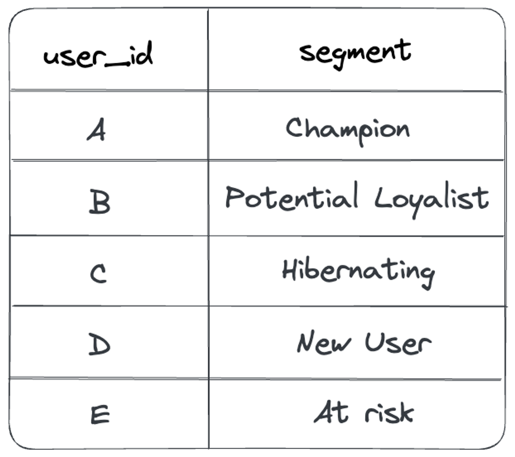
• If you are running a retention campaign and you are prioritizing your “Champions”, are you able to check if they are still “Champions” a month after you contacted them? With the model proposed before, you can’t verify if a Champion is still a champion because you only keep the customer’s last status.
• If you are running an activation campaign and you are prioritizing your “New Users”, you are also unable to check if they became “Champions” or if they are “Hibernating” a month later.

Code redundancy with data scientists

It might also be the case that you have a data science or machine learning (ML) team in your company. The ML practitioners often use user attributes as an input to train their models (also called features in a data science context). In order for that attribute to be useful as a feature in the ML model, they need to know how it changed over time.

As a result, data scientists often end up rewriting the same user attributes logic in their modeling language (typically Python). This results in wasted effort and inconsistency in business logic between the machine learning and the analytics engineering models.

Analytics engineering best practices are oriented to helping the data team reuse the models built by other practitioners. We need to find a way to extend that outside of just the analytics team and impact the data team as a whole.

Solution

The approach to solving this is quite simple; we need to build a model that doesn’t just consider the last value for each user attribute, but instead saves a snapshot of how it changed over time.

One way to solve it would be to use dbt snapshots, but this would only keep the attributes history from the time of our model deployment onwards, losing potentially useful data that existed prior to that point in time.

A better approach for our use case was to calculate the snapshots in our SQL logic. This snapshot can be calculated in various time windows (monthly, weekly, daily) depending on the type of analysis that you need to perform.

In this section we’ll show you how to build a basic user segmentation model with RFM that only keeps the current value, and then we will go through the changes in the code to preserve the segmentation history.

RFM Segmentation

The goal of RFM analysis is to segment customers into groups based on how recently they made a purchase (Recency), how frequently they make purchases (Frequency), and how much money they spend (Monetary).

We are going to use just the Recency and Frequency matrix, and use the Monetary value as an accessory attribute. This is a common approach in companies where the Frequency and the Monetary Value are highly correlated.

Example of a Recency and Frequency matrix

RFM model for current segment

We will first use a SELECT * CTE to load all our payments data. The columns that we will be using for the segmentation are the following:

• user_id: Unique identifier for each user or customer
• payment_date: Date of each customer’s payment
• payment_id: Unique identifier of each payment
• payment_amount: Transacted amount of each payment

WITH payments AS(
    SELECT *
    FROM ref {{'fact_payments'}}
),

user_id	payment_date	payment_id	payment_amount
A	2022-11-28 14:41:45	AA	2588.35
B	2022-11-28 14:42:37	BB	10104.99
C	2022-11-28 14:42:51	CC	2588.35
D	2022-11-28 14:43:42	DD	580.5
E	2022-11-28 14:44:44	EE	462.36

Next we will calculate the RFM (recency, frequency and monetary value) for each user:

• max_payment_date: Last payment date of each user. We keep it for auditing
• recency: Days that passed between the last transaction of each user and today
• frequency: Quantity of user transactions in the analyzed window
• monetary: Transacted amount by the user in the analyzed window

rfm_values AS (
    SELECT  user_id,
            MAX(payment_date) AS max_payment_date,
            NOW() - MAX(payment_date) AS recency,
            COUNT(DISTINCT payment_id) AS frequency,
            SUM(payment_amount) AS monetary
    FROM payments
    GROUP BY user_id
),

user_id	max_payment_date	recency	frequency	monetary
A	2023-04-20 10:22:39	4 18:20:22.034	4	83686.65
B	2023-04-20 10:56:15	4 17:46:46.034	13	53196.06
C	2023-04-24 13:19:18	0 15:23:43.034	22	56422.6
D	2023-04-19 19:00:24	5 09:42:37.034	4	2911.16
E	2023-03-23 19:22:00	32 09:21:01.034	40	30595.15

There are various approaches to dividing users based on their RFM values. In this model we use percentiles to divide customers into groups based on their relative ranking in each of the three metrics, using the PERCENT_RANK() function.

rfm_percentiles AS (
    SELECT  user_id,
            recency,
            frequency,
            monetary,
            PERCENT_RANK() OVER (ORDER BY recency DESC) AS recency_percentile,
            PERCENT_RANK() OVER (ORDER BY frequency ASC) AS frequency_percentile,
            PERCENT_RANK() OVER (ORDER BY monetary ASC) AS monetary_percentile
    FROM rfm_values
),

user_id	recency	frequency	monetary	recency_percentile	frequency_percentile	monetary_percentile
A	44 22:06:59.615	8	960.01	0.65	0.75	0.5
B	421 15:21:49.829	13	2348.49	0.09	0.84	0.78
C	1 15:04:48.922	7	3532.08	0.97	0.71	0.81
D	4 21:16:33.112	4	490.14	0.91	0.56	0.34
E	2 08:08:22.921	14	7239.69	0.95	0.85	0.28

Now that we have the percentiles of each RFM value of each user, we can assign them a score based on were they end up on the distribution, going by steps of 0.2 or 20% each:

• recency_score: Recency percentile values grouped from 1 to 5
• frequency_score: Frequency percentile values grouped from 1 to 5
• monetary_score: Monetary percentile values grouped from 1 to 5

rfm_scores AS(
    SELECT  *,
            CASE
                WHEN recency_percentile >= 0.8 THEN 5
                WHEN recency_percentile >= 0.6 THEN 4
                WHEN recency_percentile >= 0.4 THEN 3
                WHEN recency_percentile >= 0.2 THEN 2
                ELSE 1
                END AS recency_score,
            CASE
                WHEN frequency_percentile >= 0.8 THEN 5
                WHEN frequency_percentile >= 0.6 THEN 4
                WHEN frequency_percentile >= 0.4 THEN 3
                WHEN frequency_percentile >= 0.2 THEN 2
                ELSE 1
                END AS frequency_score,
            CASE
                WHEN monetary_percentile >= 0.8 THEN 5
                WHEN monetary_percentile >= 0.6 THEN 4
                WHEN monetary_percentile >= 0.4 THEN 3
                WHEN monetary_percentile >= 0.2 THEN 2
                ELSE 1
                END AS monetary_score
    FROM rfm_percentiles
),

user_id	recency_percentile	frequency_percentile	monetary_percentile	recency_score	frequency_score	monetary_score
A	0.26	0.3	0.12	2	2	1
B	0.94	0.38	0.23	5	2	2
C	0.85	0.96	0.87	5	5	5
D	0.71	0.63	0.93	4	4	5
E	0.67	0.51 lo	0.76	4	3	5

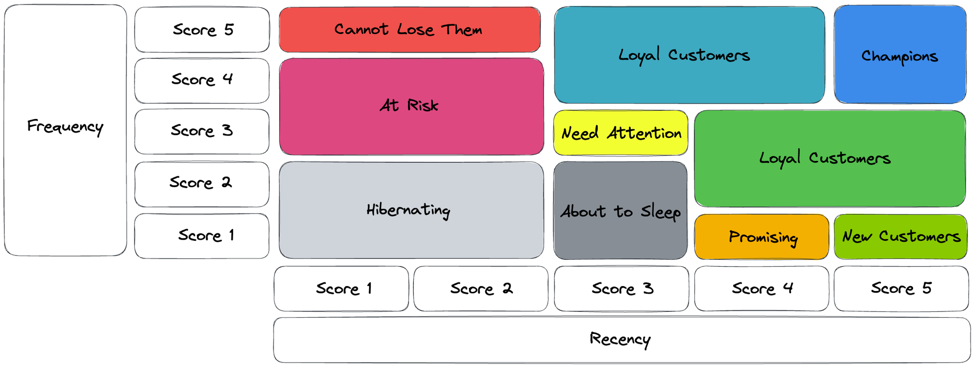
Lastly, we can segment the users by their frequency and recency scores based on the proposed R-F matrix:

• rfm_segment: Segment of each user based on a mapping of the recency and frequency scores.

rfm_segment AS(
SELECT *,
        CASE
            WHEN recency_score <= 2
                AND frequency_score <= 2 THEN 'Hibernating'
            WHEN recency_score <= 2
                AND frequency_score <= 4 THEN 'At Risk'
            WHEN recency_score <= 2
                AND frequency_score <= 5 THEN 'Cannot Lose Them'
            WHEN recency_score <= 3
                AND frequency_score <= 2 THEN 'About to Sleep'
            WHEN recency_score <= 3
                AND frequency_score <= 3 THEN 'Need Attention'
            WHEN recency_score <= 4
                AND frequency_score <= 1 THEN 'Promising'
            WHEN recency_score <= 4
                AND frequency_score <= 3 THEN 'Potential Loyalists'
            WHEN recency_score <= 4
                AND frequency_score <= 5 THEN 'Loyal Customers'
            WHEN recency_score <= 5
                AND frequency_score <= 1 THEN 'New Customers'
            WHEN recency_score <= 5
                AND frequency_score <= 3 THEN 'Potential Loyalists'
            ELSE 'Champions'
        END AS rfm_segment
FROM  rfm_scores
)
SELECT *
FROM rfm_segment

user_id	recency_score	frequency_score	monetary_score	rfm_segment
A	4	3	5	Potential Loyalists
B	4	5	5	Loyal Customers
C	5	4	5	Champions
D	1	5	5	Cannot Lose Them
E	1	4	5	At Risk

RFM model with segmentation history

This next example shows how you can build a model with a snapshot of the user attributes at the end of each month. The same could be built for a weekly model with minor adjustments.

WITH payments AS(
    SELECT *
    FROM ref {{'fact_payments'}}
),
months AS(
    SELECT NOW() AS date_month
    UNION ALL
    SELECT DISTINCT date_month AS date_month
    FROM ref {{'dim_calendar'}}
),
payments_with_months AS(
    SELECT  user_id,
            date_month,
            payment_date,
            payment_id,
            payment_amount
    FROM months
        JOIN payments ON payment_date <= date_month 
),
rfm_values AS (
    SELECT  user_id,
            date_month,
            MAX(payment_date) AS max_payment_date,
            date_month - MAX(payment_date) AS recency,
            COUNT(DISTINCT payment_id) AS frequency,
            SUM(payment_amount) AS monetary
    FROM payments_with_months
    GROUP BY user_id, date_month
),
rfm_percentiles AS (
    SELECT  user_id,
            date_month,
            recency,
            frequency,
            monetary,
            PERCENT_RANK() OVER (ORDER BY recency DESC) AS recency_percentile,
            PERCENT_RANK() OVER (ORDER BY frequency ASC) AS frequency_percentile,
            PERCENT_RANK() OVER (ORDER BY monetary ASC) AS monetary_percentile
    FROM rfm_values
),
rfm_scores AS(
    SELECT  *,
            CASE
                WHEN recency_percentile >= 0.8 THEN 5
                WHEN recency_percentile >= 0.6 THEN 4
                WHEN recency_percentile >= 0.4 THEN 3
                WHEN recency_percentile >= 0.2 THEN 2
                ELSE 1
                END AS recency_score,
            CASE
                WHEN frequency_percentile >= 0.8 THEN 5
                WHEN frequency_percentile >= 0.6 THEN 4
                WHEN frequency_percentile >= 0.4 THEN 3
                WHEN frequency_percentile >= 0.2 THEN 2
                ELSE 1
                END AS frequency_score,
            CASE
                WHEN monetary_percentile >= 0.8 THEN 5
                WHEN monetary_percentile >= 0.6 THEN 4
                WHEN monetary_percentile >= 0.4 THEN 3
                WHEN monetary_percentile >= 0.2 THEN 2
                ELSE 1
                END AS monetary_score
    FROM rfm_percentiles
),
rfm_segment AS(
SELECT *,
        CASE
            WHEN recency_score <= 2
                AND frequency_score <= 2 THEN 'Hibernating'
            WHEN recency_score <= 2
                AND frequency_score <= 4 THEN 'At Risk'
            WHEN recency_score <= 2
                AND frequency_score <= 5 THEN 'Cannot Lose Them'
            WHEN recency_score <= 3
                AND frequency_score <= 2 THEN 'About to Sleep'
            WHEN recency_score <= 3
                AND frequency_score <= 3 THEN 'Need Attention'
            WHEN recency_score <= 4
                AND frequency_score <= 1 THEN 'Promising'
            WHEN recency_score <= 4
                AND frequency_score <= 3 THEN 'Potential Loyalists'
            WHEN recency_score <= 4
                AND frequency_score <= 5 THEN 'Loyal Customers'
            WHEN recency_score <= 5
                AND frequency_score <= 1 THEN 'New Customers'
            WHEN recency_score <= 5
                AND frequency_score <= 3 THEN 'Potential Loyalists'
            ELSE 'Champions'
        END AS rfm_segment
FROM  rfm_scores
)
SELECT *
FROM rfm_segment

The original query uses the current date (obtained by using the NOW() function) to calculate the recency of each user, whereas the new approach includes 2 CTEs that allow the RFM scores to be calculated on a monthly basis.

• The first CTE queries a calendar table and selects the date_month column. It also appends a row with the NOW() function to calculate the attributes for the current month.

months AS(
    SELECT NOW() AS date_month
    UNION ALL
    SELECT DISTINCT date_month AS date_month
    FROM ref {{'dim_calendar'}}
),

date_month
2023-04-25 5:51:09
2023-04-01 0:00:00
2023-03-01 0:00:00
2023-02-01 0:00:00
2023-01-01 0:00:00

• The second CTE has a LEFT JOIN that keeps the list of payments the user had until the end of each month, which allows the model to calculate the RFM segment the user had at the end of each period.
• The recency metric is calculated to the end of each month. If the month is not yet finished, we calculate it to the current day (thanks to the UNION in the first query).

payments_with_months AS(
    SELECT  user_id,
            date_month,
            payment_date,
            payment_id,
            payment_amount
    FROM months
        JOIN payments ON payment_date <= date_month 
),

user_id	date_month	payment_date	payment_id	amount
A	2023-04-25 5:55:05	2022-04-16 19:41:05	BB	120
A	2023-04-25 5:55:05	2023-03-23 18:17:46	AA	160
A	2023-04-01 0:00:00	2023-03-23 18:17:46	AA	160
B	2023-04-25 5:55:05	2022-08-23 17:52:44	CC	90
B	2023-04-01 0:00:00	2022-08-23 17:52:44	CC	90
E	2023-04-25 5:55:05	2023-02-05 12:17:19	EE	10630
E	2023-04-01 0:00:00	2023-02-05 12:17:19	EE	10630

Getting the lastest status

Once we have our historical model built, we can add another model that runs after it in our dependency graph. This can help reduce the latency in use cases where querying the whole history is not needed (like personalization initiatives).

WITH rfm_segments AS(
    SELECT *
    FROM ref {{'model_rfm_segments_hist'}}
),  
current_segments AS(
    SELECT *
    FROM rfm_segments
    WHERE date_month = (SELECT MAX(date_month) FROM rfm_segments)
)
SELECT *
FROM current_segments

Solution overview

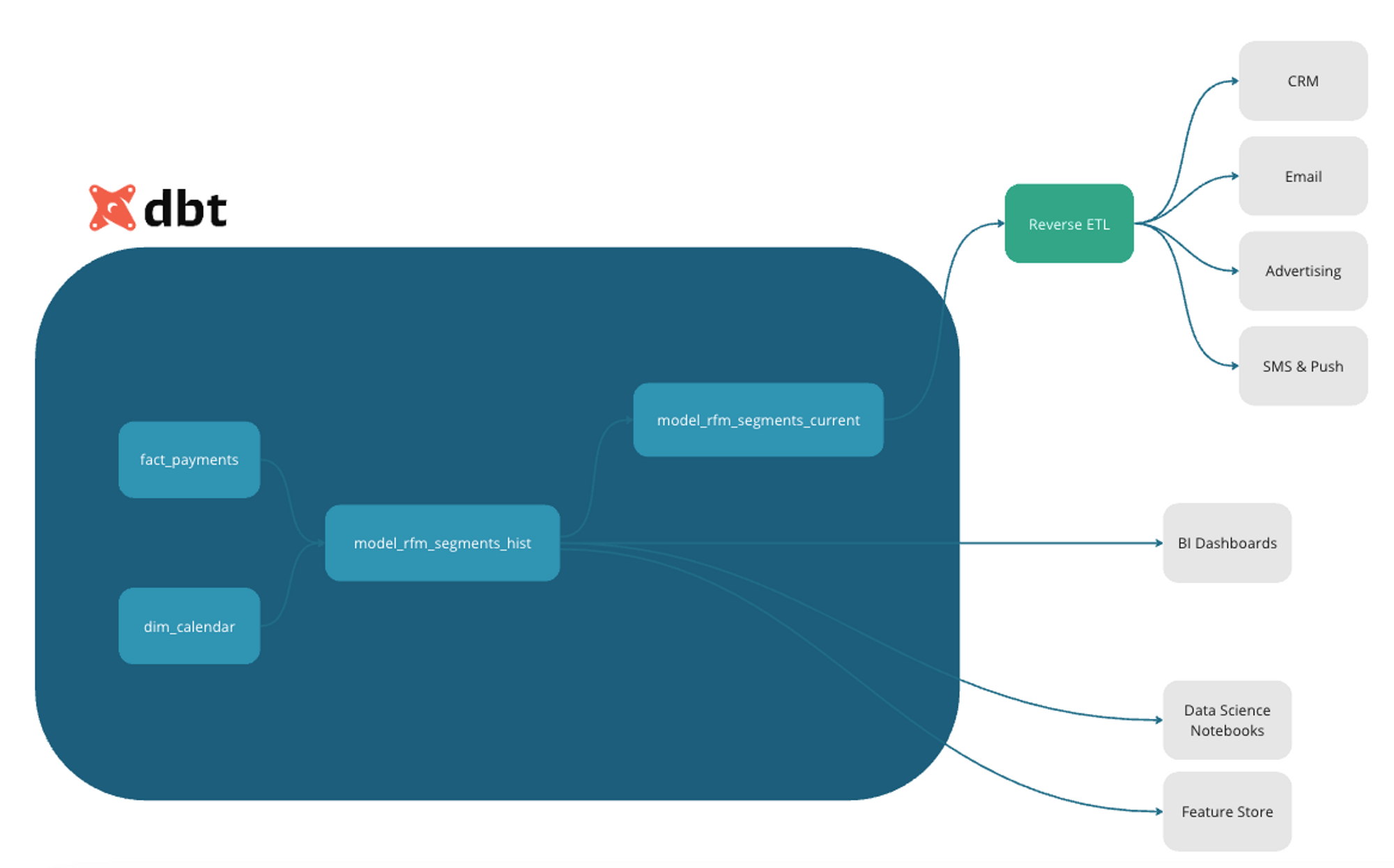
With the new approach, our dependency graph would look like this:

RFM models dependency graph

• For analysts that want to see how the segments changed over time, they can query the historical model. There is also an option to build an aggregated model before loading it in a Business Intelligence tool.
• For ML model training, data scientists and machine learning practitioners can import this model into their notebooks or their feature store, instead of rebuilding the attributes from scratch.
• If you want to personalize the experience of a user based on their segment, like in the CX example from the beginning, you can query the current segmention and export it to your CRM with a Reverse ETL tool.

Conclusions

This design has trade-offs, notably longer build-time and harder explainability. However, we believe that data teams that invest in this approach will get better datasets for historical analysis, more collaboration with data scientists, and overall greater impact from their analytics engineering efforts.

Related resources

Operational Analytics in Practice

How dbt Labs' data team approaches reverse ETL

The Operational Data Warehouse: Reverse ETL, CDPs, and the future of data activation